Diffusion Models

Before diffusion models, image generation was largely dominated by GANs. This was despite their inherently poor training stability caused by their two competing networks. Diffusion models emerged as a more stable alternative that produce highly realistic images, and now, are the most popular model for image generation tasks. But what are diffusion models, and how do they work?

What are diffusion models?

Diffusion models are a type of generative model that learn how to transform noise into real images. They are trained by adding various amounts of random noise to images, and learning how to undo the added noise. After training, a diffusion model can transform a pure noise input into a realistic image.

Diffusion models (DDPMS) were introduced by Sohl-Dickstein et al. (2015) and popularized through Ho et al’s “Denoising Diffusion Probabilistic Models”. DDPMs have two key functionalities: the forward process, and the reverse process.

Forward Process

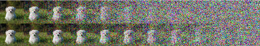
The forward (diffusion) process gradually adds Gaussian noise to an input image over a total of $T$ timesteps. At each timestep, the amount of noise for the current image $x_t$ is computed with:

$$q(\mathbf{x}_t|\mathbf{x}_0) = \mathcal{N}(\mathbf{x}_t; \sqrt{\bar{\alpha}_t}\mathbf{x}_0, (1 - \bar{\alpha}_t)\mathbf{I})$$

$\alpha_t$ represents the amount of signal, or non-noise, in the image. Conversely, the intensity of the noise at the current timestep $1 - \alpha_t = \beta_T$ is controlled by a noise scheduler. Ho et al. utilized a linear noise scheduler, which creates $T$ equally incremented values of $\beta_T$ from 1e-4 to 0.02. Larger timesteps produce larger $\beta_T$ values, which increasingly corrupt the input image. However, a linear scheduler produces high $\beta_T$ values for many timesteps, producing a larger portion of degraded images that are less useful to train with. Nichol & Dhariwal later proposed a cosine noise scheduler that increments $\beta_T$ more gradually to provide more informative data samples, consequently improving image generations.

Rather than computing each noisy step sequentially, the forward process can be reparameterized so we can jump directly to any timestep. We can represent $X \sim \mathcal{N}(\mu, \sigma^2)$ as $X = \mu + \sigma\epsilon$, $\epsilon \sim \mathcal{N}(0, 1)$, which means we can represent $\mu$ as $\bar{\alpha}_t x_0$, and $\sigma^2 = (1 - \bar{\alpha}_t)$, so $\sigma = \sqrt{1 - \bar{\alpha}_t}$, where $\alpha_T$ represents the amount of signal $(1 - \beta_T)$. Plugging into $\mu + \sigma\epsilon$, we get

$$x_t = \sqrt{\bar{\alpha}_t}\, x_0 + \sqrt{1 - \bar{\alpha}_t}\, \epsilon \tag{2}$$

where $\epsilon$ is sampled from Gaussian noise. The model then attempts to predict the added noise $\epsilon$ at the current timestep. To learn how to predict the added noise $\epsilon$, the model is trained with the loss term:

$$L_{\text{simple}}(\theta) := \mathbb{E}_{t, \mathbf{x}_0, \epsilon} \left[ \|\epsilon - \epsilon_\theta(\sqrt{\bar{\alpha}_t}\mathbf{x}_0 + \sqrt{1 - \bar{\alpha}_t}\epsilon, t)\|^2 \right] \tag{3}$$

which is essentially MSE loss between the true noise and the predicted noise. Interestingly, this loss term is actually a simplified version of the original term:

$$\mathbb{E}_{\mathbf{x}_0, \epsilon} \left[ \frac{\beta_t^2}{2\sigma_t^2 \alpha_t(1 - \bar{\alpha}_t)} \|\epsilon - \epsilon_\theta(\sqrt{\bar{\alpha}_t}\mathbf{x}_0 + \sqrt{1 - \bar{\alpha}_t}\epsilon, t)\|^2 \right] \tag{4}$$

The original objective penalizes the model heavily for incorrect predictions on later timesteps (noisier images) so it can prioritize learning from difficult-to-denoise images. However, Ho et al. determined that the simplified loss term produces better quality samples.

Reverse Process

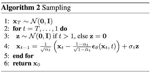
The reverse process undoes the forward process through a Markov chain, meaning that an image's next slightly-less noised state depends on the current noise. For each timestep, reverse diffusion slightly undoes the noise of the image until a clean image is produced. After the network predicts $\epsilon$ from image $X_t$, we can compute the mean of the distribution of $X_{t-1}$ with

$$\boldsymbol{\mu}_\theta(\mathbf{x}_t, t) = \tilde{\boldsymbol{\mu}}_t\left(\mathbf{x}_t, \frac{1}{\sqrt{\bar{\alpha}_t}}(\mathbf{x}_t - \sqrt{1 - \bar{\alpha}_t}\epsilon_\theta(\mathbf{x}_t))\right) = \frac{1}{\sqrt{\alpha_t}}\left(\mathbf{x}_t - \frac{\beta_t}{\sqrt{1 - \bar{\alpha}_t}}\epsilon_\theta(\mathbf{x}_t, t)\right) \tag{5}$$

We can then find $X_{t-1}$ with

$$x_{t-1} = \frac{1}{\sqrt{\alpha_t}} \left( x_t - \frac{1 - \alpha_t}{\sqrt{1 - \bar{\alpha}_t}} \epsilon_\theta(x_t, t) \right) + \sigma_t z, \tag{6}$$

where $z \sim \mathcal{N}(0, I)$ if $t > 1$, else $z = 0$. When $t = 0$, that is the very last step of the reverse process, which is where the noiseless image is produced.

Model Architectures

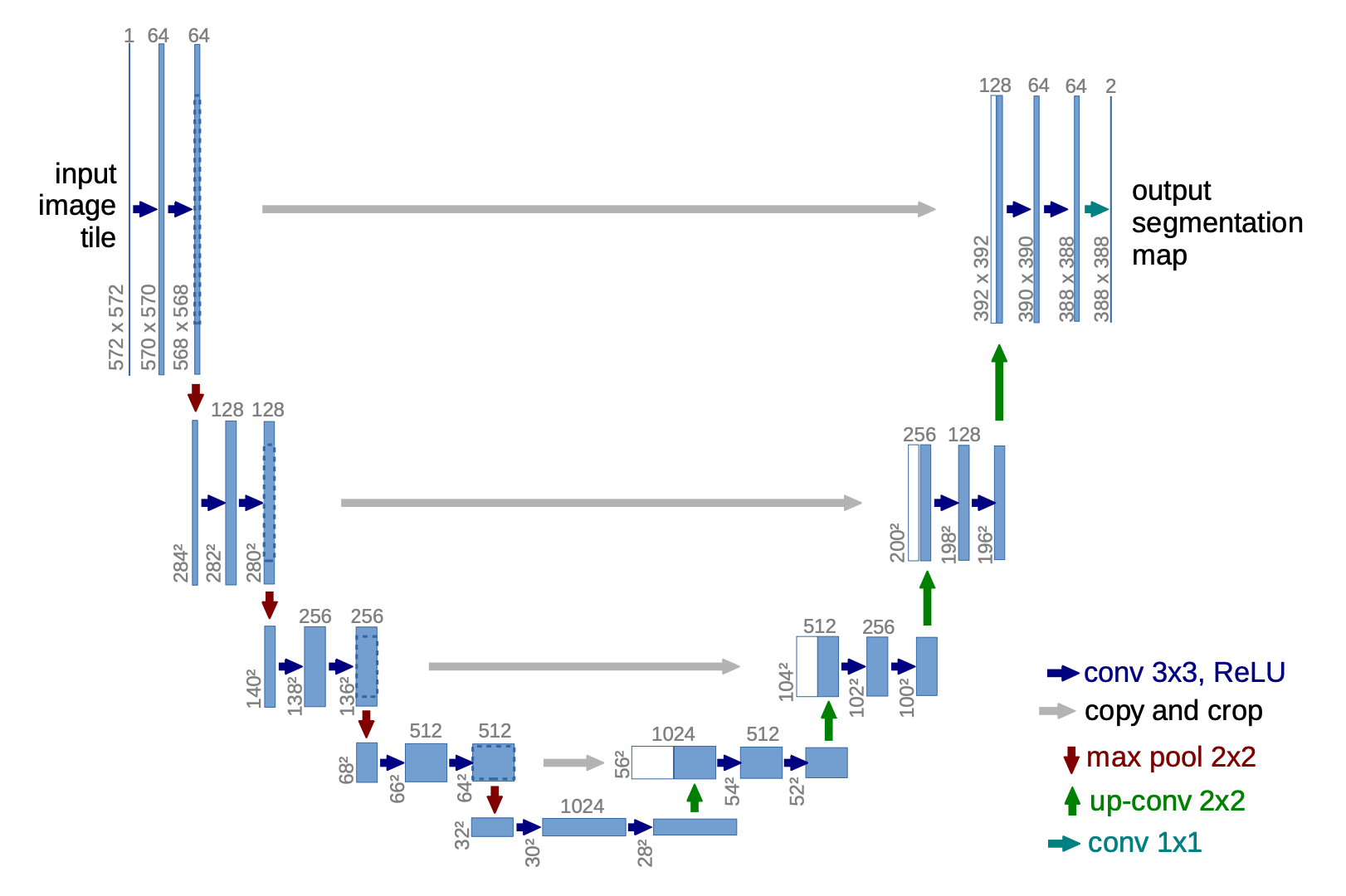
To perform the noise prediction, Ho et al. (2021) utilized a modified U-Net model (Ronneberger et al., 2015). U-Net consists of a decoder, bottleneck, and encoder, with skip connections between layers of the same resolution in the encoder and decoder.

The U-Net is time-conditioned using the current timestep so the model can understand that larger timesteps correspond with noisier images. However, the timestep $T$ is not directly passed through the model because a single large integer timestep value is not informative or efficient for the model to process. Timesteps are embedded using Transformer sinusoidal positional embeddings (Vaswani et al., 2017), which turn the single integer into a vector of size $d_{model}$ that is computed with:

$$PE_{(pos, 2i)} = \sin(pos / 10000^{2i/d_{\text{model}}}) \tag{7}$$ $$PE_{(pos, 2i+1)} = \cos(pos / 10000^{2i/d_{\text{model}}}) \tag{8}$$

Cosine and sine are utilized for computing positional embeddings because they allow timestep $t$ to be a linear transformation of timestep $t + k$, which allows the model to learn the relative positions between timesteps with ease. Neither cosine and sine can individually be used because when we represent the embedding as a point in a 2D unit circle, shifting $k$ timesteps requires both cosine and sine shifts. Additionally, a huge benefit of representing the timestep with sinusoidal positional embeddings is they are deterministic. No training is required to produce them.

The U-Net's blocks consist of two residual layers (He et al., 2015), with two residual blocks per image resolution. The U-Net also includes self-attention blocks (Vaswani et al., 2017) at the bottleneck and 16x16 resolution layers. These self-attention blocks pass feature maps through three linear projections ($W_Q$, $W_K$, and $W_V$) to produce queries ($Q$), keys ($K$), and values ($V$). Attention weights are then computed as:

$$\mathrm{Attention}(Q, K, V) = \mathrm{softmax}\!\left(\frac{QK^\top}{\sqrt{d_k}}\right)V$$

While it is unclear exactly what relationship the self-attention blocks create between pixels of a feature map, they improve denoising capabilities because they help the model create relationships between any region of a feature map. Convolutional blocks alone are insufficient for diffusion because they only learn local relationships due to their small kernel sizes.

An alternative to the U-Net in diffusion models emerged with Diffusion Transformers (DiTs) (Peebles & Xie, 2022), where a vision transformer (ViT) replaces the U-Net. The flow of a DiT is: compress an input image with a VAE encoder into a latent representation $z$, noise $z$, and patch $z$ with the ViT before performing forward diffusion. The benefit of using a transformer instead of an attention-based UNet is because transformers are more scalable. Larger transformers empirically perform better at diffusion generation than similarly sized UNets (Peebles & Xie, 2022).

Guided diffusion

As is, diffusion models produce diverse, uncontrollable outputs. Their generations are inherently probabilistic because their inference step begins with random noise. Diffusion models can have their outputs be guided towards a specific class or result through several methods. Basic conditioning simply involves concatenating or cross-attending $y$ (a condition image or text label) with the input before it is passed through the diffusion model. In the case of text label conditioning, the text and image must both be converted to embeddings through CLIP encoders before passing through the diffusion model.

Dhariwal & Nichol (2021) introduced classifier guided diffusion, where they train a classifier model on noisy images from forward diffusion, and use their gradients to guide the noise prediction towards the target conditioning class $y$.

Ho & Salimans (2022) introduced classifier-free diffusion guidance, where instead of training a separate classifier, a diffusion model that is simultaneously conditioned and unconditioned is trained. During training, the condition $c$ can be randomly dropped. During inference, both conditioned and unconditioned predictions are obtained for an input sample, and the final sample is guided using:

$$\tilde{\epsilon}_\theta(\mathbf{z}_\lambda, \mathbf{c}) = (1 + w)\epsilon_\theta(\mathbf{z}_\lambda, \mathbf{c}) - w\epsilon_\theta(\mathbf{z}_\lambda) \tag{9}$$

Where $w$ is a weight that when increased, guides the generation towards the conditioned prediction while decreasing sample diversity.

Training

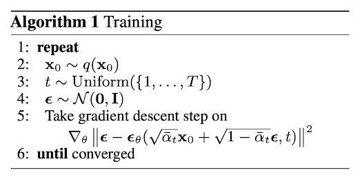
The flow of training a diffusion model is as follows for an input training sample $x$:

1. Randomly select a timestep value between 0 and $T$. $T = 1000$ is a common choice.
2. Add noise to input $x_t$ with equation (2)
3. Pass the noised image, and condition if using a conditional diffusion model, into the model. Return the predicted noise $\epsilon$.
4. Pass the predicted noise $\epsilon$ and the actual noise to the loss function.
5. Perform backprop.

Inference: DDPM vs. DDIM

After the diffusion model has been trained, we can input an image consisting of total noise (alongside potential conditioning) to the model, perform reverse diffusion, and produce realistic data samples. DDPM inference, however, is extremely time-consuming and compute-intensive: for all timestep values, we have to predict a denoised image. For 1000 timesteps, that means 1000 consecutive denoising operations.

Song et al. introduced denoising diffusion implicit models (DDIMs), which reparameterize the Markovian forward and reverse process to become non-Markovian. The reverse process is represented as:

$$\mathbf{x}_{t-1} = \sqrt{\alpha_{t-1}} \underbrace{\left(\frac{\mathbf{x}_t - \sqrt{1 - \alpha_t}\epsilon_\theta^{(t)}(\mathbf{x}_t)}{\sqrt{\alpha_t}}\right)}_{\text{"predicted } \mathbf{x}_0\text{"}} + \underbrace{\sqrt{1 - \alpha_{t-1} - \sigma_t^2} \cdot \epsilon_\theta^{(t)}(\mathbf{x}_t)}_{\text{"direction pointing to } \mathbf{x}_t\text{"}} + \underbrace{\sigma_t \epsilon_t}_{\text{random noise}} \tag{10}$$

At each inference step, we can directly predict the clean image $x_0$ with our current image and the predicted $\epsilon$. Since we can jump directly to the cleaner image without requiring consecutive renoising steps, inference can be accelerated by taking large timestep jumps with little loss in generation quality. DDIM can reduce the 1000 timesteps of DDPM inference to ~50 steps. Because DDPMs also predict $\epsilon$, we can use DDIM inference on DDPM-trained models.

References

1. Sohl-Dickstein et al. (2015). Deep unsupervised learning using nonequilibrium thermodynamics. arXiv

2. Ho et al. (2020). Denoising diffusion probabilistic models (DDPM). arXiv

3. Nichol & Dhariwal (2021). Improved denoising diffusion probabilistic models. arXiv

4. Ronneberger et al. (2015). U-Net: Convolutional networks for biomedical image segmentation. arXiv

5. Vaswani et al. (2017). Attention is all you need. arXiv

6. He et al. (2015). Deep residual learning for image recognition (ResNet). arXiv

7. Dosovitskiy et al. (2020). An image is worth 16×16 words (Vision Transformer). arXiv

8. Peebles & Xie (2022). Scalable diffusion models with transformers (DiT). arXiv

9. Dhariwal & Nichol (2021). Diffusion models beat GANs on image synthesis (ADM). arXiv

10. Ho & Salimans (2022). Classifier-free diffusion guidance. arXiv

11. Song et al. (2020). Denoising diffusion implicit models (DDIM). arXiv