MeanFlow One-Step Generation

Flow matching models are a type of generative model that shift one data distribution to another by learning the velocity field between the two. They are trained to learn the instantaneous velocity of data samples at a timestep between $t = 0$ (the initial data distribution) and $t = 1$ (the final data distribution). Generating data from a trained flow matching model involves taking a sample from the initial distribution (like a Gaussian), integrating the velocity field step-by-step from $t = 0$ to $t = 1$, and shifting the sample towards the target distribution through the integrated displacement path. However, flow matching can be computationally expensive because the quality of the final sample generally improves with more integration steps.

MeanFlow: what is it and why is it important?

MeanFlow fixes this by providing single-step generation. Instead of learning the instantaneous velocity of many points between two distributions, MeanFlow learns the average velocity field of two times, $r$ and $t$, between two distributions directly, which allows jumping from one distribution to another in one step [1].

$$u(z_t, r, t) = v(z_t, t) - (t - r)\frac{d}{dt}\bigl[u(z_t, r, t)\bigr]$$

The above MeanFlow identity states that average velocity $u$ between times $r$ and $t$ can be represented by the instantaneous velocity and the rate of change of the average velocity between $r$ and $t$. However, because $u$ is represented by a neural network, computing the derivative of $u$ requires expensive Jacobian calculations. To perform the derivative efficiently, MeanFlow uses a Jacobian-vector product (JVP) to compute the directional derivative of $u$ for only the input state $z_t$, which is much less computationally intensive. MeanFlow is able to evaluate the derivative of $u$ with a JVP instead of a full Jacobian because the derivative of $du/dt$ with respect to $z_t$, $r$, and $t$ becomes

$$\frac{d}{dt}u(z_t, r, t) = \frac{dz_t}{dt}\partial_{z_t}u + \frac{dr}{dt}\partial_r u + \frac{dt}{dt}\partial_t u$$

In this setup, $dz_t/dt = v(z_t, t)$, $dr/dt = 0$ (because $r$ is held constant in the JVP direction), and $dt/dt = 1$. Substituting these gives:

$$\frac{d}{dt}u(z_t, r, t) = v(z_t, t)\partial_{z_t}u + \partial_t u$$

Torch's torch.func.jvp can efficiently perform the JVP between vector $V$ and Jacobian matrix $u$.

MeanFlow Implementation

I implemented a MeanFlow model with a UNet backbone and uniform distribution timestep sampler using the paper and source code as reference [1][2].

Timestep sampling and embedding

A vital part of MeanFlow is the method of sampling for timesteps $r$ and $t$ during training. The MeanFlow paper experimented with sampling from uniform and lognorm distributions, and achieved the best results from lognorm [1]. I sampled from a uniform distribution between 0 and 1 due to the simplicity of its implementation. To satisfy the condition that timestep $r$ is $\leq t$, my sampler first creates tensor $t$ of shape $([batchsize])$ with random values within 0 and 1, then created tensor $r$ of the same shape and distribution, except it is scaled by $t$ ($r \cdot t$). Since $t$ is between 0 and 1, $r$'s elements would be scaled to always be less than or equal to $t$'s elements.

The authors also ensure that a certain percentage of all $(r, t)$ sample pairs had $r \neq t$. I chose 25% because the paper achieved their best results with that ratio [1]. I enforced this ratio by creating a mask that randomly chooses 25% of $r$'s tensor to be False, and used torch.where to turn all false $r$ elements to the corresponding $t$ element. I utilized their source code as a reference for the sampler's implementation [2].

After the timesteps are sampled, they must be embedded in order to condition the backbone model. I chose sinusoidal positional embeddings because they are quick to compute and do not require any training [6]. I initially wanted to embed $r$ and $t$ separately and combine their embeddings, but the paper says they "achieved the best results with embedding $(t, t-r)$, that is, time and interval, achieves the best result, while directly embedding $(r, t)$ performs almost as well", so I decided to condition with $(t, t - r)$. After embedding $t$ and $t-r$, I passed both embeddings through an MLP (as MeanFlow's source code does) before combining them. I implemented the sinusoidal embeddings from reference [1][2].

Backbone

In my MeanFlow implementation, I chose a UNet backbone instead of a DiT or ViT because I wanted to start with a smaller architecture and I was already familiar with UNet from previous segmentation projects [5]. My UNet consisted of residual blocks [4] with two sets of convolutions and a skip connection for improved training stability. The encoder and decoder used 3 residual blocks each, which span the resolutions $64 \times 64$, $32 \times 32$, $16 \times 16$, and $8 \times 8$. I chose these resolutions because I preprocessed my dataset to be cropped to $64 \times 64$ images, and I thought going down to $8 \times 8$ was a good initial tradeoff between feature map amount and computational load. The UNet is conditioned with timesteps $r$ and $t$, which are embedded via sinusoidal positional embeddings and injected between the convolutional layers of the residual blocks. However, while I was planning on also conditioning the UNet with image labels, I unfortunately ran out of time to do so. I wrote the UNet from scratch, and used Cursor to double check my code.

Loss Function

I trained the model with an MSE objective between the predicted average velocity and the target average velocity:

$$L(\theta) = \mathbb{E}\bigl[u_\theta(z_t, r, t) - \mathrm{sg}(u_{\mathrm{tgt}})^2\bigr]$$

In my implementation, this is the MSE loss between $u_\theta(z_t, r, t)$ and $u_{\mathrm{tgt}}$. Note that the $\mathrm{sg}$ term means that no gradients flow through the target average velocity during backpropagation. I use .detach() to achieve this in my implementation: train_loss = loss_fn(u, u_tgt.detach()).

Image Sampler/Inference

For inference, I followed their one-step sampling method. The idea is to jump directly between two timesteps with one model evaluation of the MeanFlow network [1].

$$z_r = z_t - (t - r)u_\theta(z_t, r, t)$$

I implemented this equation in inference.py using the same setup as their reference approach: sample a starting latent, choose $r$ and $t$ for the one-step transition, run the model once to predict $u_\theta$, and apply the update above to get the final sample [2].

Dataset

I trained the UNet with ImageNette-2 [3], a 10-class subset of ImageNet. I resized each image to $64 \times 64$ for reduced computational load without losing too much detail, and normalized pixel values.

Implementation Steps

The entire process of my MeanFlow implementation, in order:

1. Created data.py to explore data samples.
2. Implemented an unconditioned UNet backbone with residual blocks.
3. Modified the UNet to be conditioned with $r$ and $t$ embeddings, and implemented sinusoidal embeddings.
4. Modified data.py to convert the training and validation sets from raw JPEGs to cropped $64 \times 64$ NPY files for faster training.
5. Implemented the timestep sampler and a training loop skeleton in train.py (minus the MeanFlow objective and JVP usage).
6. Implemented helper functions for training in utils.py (for example, loss curve plotting and experiment saving).
7. Implemented the MeanFlow objective inside the training loop, including JVP.
8. Implemented the one-step sampler in inference.py.
9. Began overfitting experiments on 3 samples (see experiment section below), and during experiments used Cursor to port training and sampling code into a single Jupyter notebook for Google Colab usage.

Implementation Issues

This section details my implementation issues, and how I fixed them.

Sampler function ratio issue

When creating the $t$ & $r$ sampler, I wanted 25% of all $(r, t)$ pairs in a batch to satisfy $r \neq t$. However, when testing the sampler with a batch size of 8, I would receive ~1–3 unequal pairs instead of the expected 2. This came from the following syntax:

mask = torch.rand(batch_size, device=device) < percent_unequal
r = torch.where(mask, t, r)

This logic does not enforce an exact percentage of unequal pairs in each batch. It applies a random threshold per element, so the unequal count can vary from batch to batch. I fixed it by correctly using torch.randperm to select an exact number of indices per batch, then building the mask from those indices so the target ratio is enforced.

Issue with MeanFlow objective

File ".../MeanFlow/train.py", line 84, in <module>
    z = (1 - t) * x + t * e
RuntimeError: The size of tensor a (3) must match the size of tensor b (64) at non-singleton dimension 3

One of the tensors had a size mismatch in this tensor operation. I thought it might be because $t$ had shape [batch_size] (with batch_size = 3 while overfitting on 3 samples), so to confirm, I printed the shape of each tensor in that equation.

t shape:  torch.Size([3])
x shape:  torch.Size([3, 3, 64, 64])
e shape:  torch.Size([3, 3, 64, 64])

To fix this, I created reshaped versions of $r$ and $t$ with shape [B, 1, 1, 1] using t_reshape = t.view(-1, 1, 1, 1) and r_reshape = r.view(-1, 1, 1, 1). That way, I could pass the original copies of $t$ and $r$ into the model, which expects shape [B] before embedding, and use the reshaped versions for image operations such as z = (1 - t_reshape) * x + t_reshape * e.

JVP tangent type error

u, dudt = torch.func.jvp(fn, (z, r, t), (v, 0, 1))
RuntimeError: jvp(f, primals, tangents): Expected tangents to only contain Tensors, got <class 'int'>

I mistakenly used integer tangents (0 and 1) instead of tensor tangents in the JVP call. I fixed this by replacing them with torch.zeros_like(t) and torch.ones_like(t).

JVP callable input error

u, dudt = torch.func.jvp(model(z, r, t), (z, r, t), (v, torch.zeros_like(t), torch.ones_like(t)))

JVP expects a callable function, but model(z, r, t) returns logits. To fix this, I created a helper function u_fn(z, t, r) in the UNet that calls model.forward(z, t, r), and passed model.u_fn into torch.func.jvp.

In-place operation error during JVP

RuntimeError: During a grad (vjp, jvp, grad, etc) transform, the function provided attempted to call in-place operation (aten::add_.Tensor) that would mutate a captured Tensor. This is not supported; please rewrite the function being transformed to explicitly accept the mutated Tensor(s) as inputs.

I found that BatchNorm layers in the UNet triggered in-place operations that were not compatible with JVP. GroupNorm worked correctly with JVP, so I replaced all BatchNorm layers with GroupNorm.

Slow early convergence

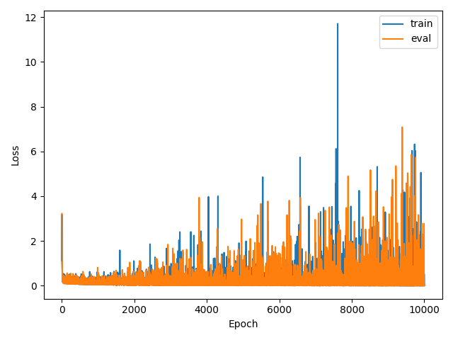
In my earlier experiments, I initially thought ~100–500 epochs would be enough for this large backbone and small dataset, but the model needed significantly more epochs to converge based on their loss curves. I trained with much more epochs for later experiments.

Poor generation quality

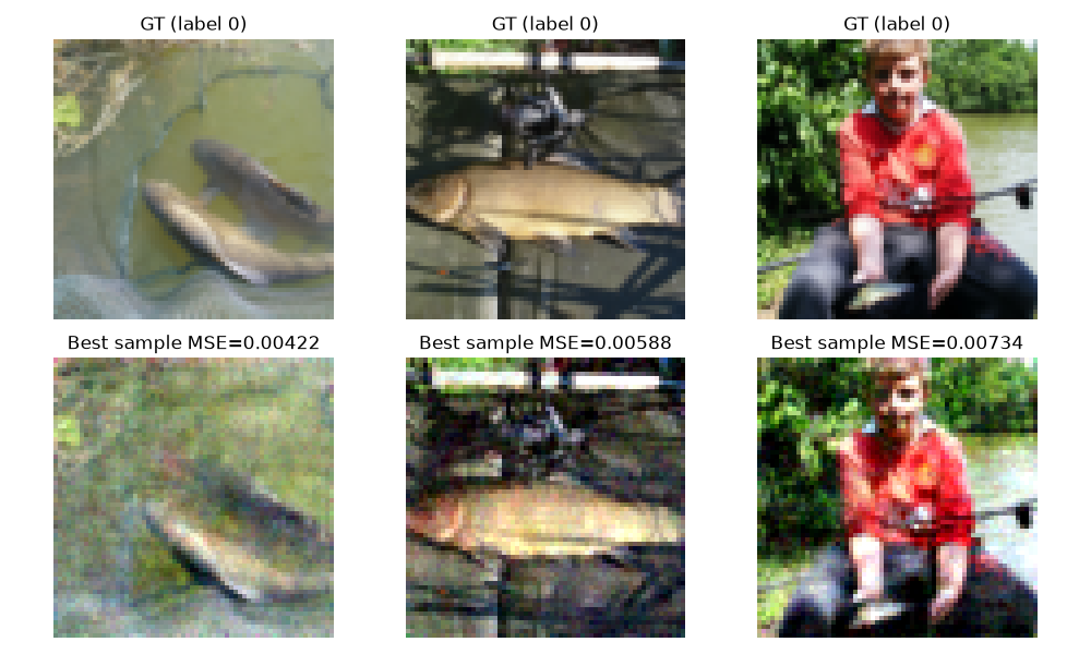
My inference script initially only produced 3 images, which looked barely anything like the real ground truth images. I realized it would be better to produce much more images (~300), and use the loss objective (MSE) as a way to choose the 3 best images to the GT, and display those. That showed me significantly better samples.

3-Sample Overfitting Experiments

Initial hyperparameters & config: 100 epochs, $1\mathrm{e}{-3}$ LR, constant LR, AdamW optimizer.

Run	Notes	Time
Run 0	Started with 100 epochs at LR 1e-3. Loss was spiky but decreasing toward convergence (~0.25), with clear room for further training. Generated images were mostly noise.	2 mins (CPU)
Run 1	Increased training to 500 epochs at LR 1e-3. Loss remained spiky but decreasing toward convergence (~0.15), with room still to go. Generated images were still mostly noise.	5 mins (CPU)
Run 2	Kept 500 epochs and lowered LR to 1e-4. Loss was still spiky but decreasing toward convergence (~0.10), with room still to go. Generated images remained mostly noise.	5 mins (CPU)
Run 3	Increased training to 1k epochs at LR 1e-3. Loss became very spiky and less stable (~0.15) and did not show smooth convergence. This run produced the weakest-looking generations.	11 mins (CPU)
Run 4	Increased training to 5k epochs at LR 1e-4. Loss remained spiky but decreasing toward convergence (~0.05), with room still to go. Generation quality improved significantly.	76 mins (CPU)
Run 5	Kept 5k epochs and changed to cosine-annealed LR from 1e-3 to 1e-5. Loss stayed spiky but decreased toward convergence (~0.02), with some room still to go. Generation quality improved.	70 mins (CPU)
Run 6	Increased training to 10k epochs with cosine-annealed LR from 1e-3 to 1e-5. Loss became low and stable near convergence (~0.001) with minimal room left to improve. This run produced the best generations and effectively overfit.	20 mins (GPU)

Results

My MeanFlow implementation successfully overfit the 3-sample training dataset by run 6, which indicates that the MeanFlow identity and sampler were implemented correctly. The loss curve was still very spiky, but I did not mind because it had effectively converged.

References

1. Geng et al. (2025). Mean Flows for One-step Generative Modeling. arXiv
2. Official MeanFlow implementation. GitHub: Gsunshine/meanflow
3. ImageNette-2 dataset. fastai/imagenette
4. He et al. (2015). Deep Residual Learning for Image Recognition. arXiv
5. Ronneberger et al. (2015). U-Net: Convolutional Networks for Biomedical Image Segmentation. arXiv
6. Vaswani et al. (2017). Attention Is All You Need. arXiv